Analysis of a Solar Thermal Beam-Powered Propulsion Rocket (and why it probably wouldn’t work)
What is a Beam-Powered Propulsion Rocket?
Conventional chemical rockets reach orbital (or faster) speeds by combusting a fuel and an oxidizer. The combustion products (typically water and CO2) are heated to 1000’s of Kelvin by the energy from the combustion process, and the turbopumps in the rocket as well as the rocket nozzle help convert the thermal energy of the combustion products into kinetic energy. The rocket then gains $\Delta v$ according to the conservation of momentum by expelling high speed combustion products. The primary disadvantage of this process is that a typical rocket will expend a signficant portion of the stored chemical energy of the propellant just accelerating the propellant (and the storage tanks for the propellant). This leaves little mass budget left over for the payload (what people are paying for) and the structure of the rocket - meaning most structures are engineered at the edge of what is possible, reducing the fatigue life of the rocket and making reusability difficult even for multi-stage vehicles. The mass of the propellant can be calculated with the Tsiolkovsky rocket equation: \(m_0=m_fe^{\Delta v / v_e}\) where $m_0$ is the wet mass (propellant + rocket), $m_f$ is the dry mass (rocket), $\Delta v$ is the change in speed the rocket achieves (usually orbital or escape velocity or a fraction of the former if multi-stage), and $v_e$ is the effective exhaust velocity. The mass of the propellant then is just $m_p = m_0-m_f$, and the effective exhaust velocity is given by: \(v_e=I_{sp}g_0\) where $g_0$ is gravitational acceleration (9.81 $m/s^2$) and $I_{sp}$ is the specific impulse, which is defined as the thrust integrated over time per unit weight (on Earth) of the propellant. $I_{sp}$ can be thought of as how efficient a rocket is at producing thrust from its propellant, with higher numbers being “better.” In general, to achieve high specific impulse, your propellant ought to be heated to as high of a temperature as possible and be as light as possible. The conventional chemical launch rocket with the highest $I_{sp}$ that has had commercial/practical applications was the Space Shuttle at 452.3 [s] in vacuum, which is close to the theoretical limit using an H2/O2 propellant. While there are other factors to consider such as specific thrust (why you probably can’t just use an ion thruster to get to orbit) and the overall cost of the system (why the Proton beat the Shuttle in cost despite being less efficient), generally increasing the $I_{sp}$ should yield a low-cost reusable vehicle. There are many alternative technologies constantly being proposed and investigated including nuclear-thermal rockets, air-breathing vehicles, sky hooks, etc. However, this article focuses on Beam-Powered Propulsion. Beam-Powered Propulsion rockets overcome the limits of chemical rockets by “beaming” the energy (or in the case of light sails and photonic laser thrusters - the reaction mass) to the rocket. The different beam-powered propulsion rockets include:
- thermal rockets: using a laser or maser (collimated microwave beam) to heat up the propellant, which avoids the mass of the oxidizer (what this article will focus on).
- Examples:
- Dr. Kevin Parkin’s Thesis
- an array of high power collimated microwave sources on the ground (gyrotrons) heat up a rocket carrying H2, CH4, or some other fuel.
- Leik Myrabo’s Light Craft
- a high powered pulsed laser explodes the air (or stored gas) of a spinning vehicle (that looks like a UFO).
- Dr. Kevin Parkin’s Thesis
- Examples:
- light sails: bouncing photons off a very reflective surface (a light sail), which imparts the momentum of the photons to the craft
- Examples:
- Breakthrough starshot
- an array of high powered lasers on Earth pushes an array of light sailed nanocrafts to Proxima Centuri.
- Breakthrough starshot
- Examples:
- photonic laser thrusters: bounces photons many times off a single surface by creating a very large laser cavity increasing the photonic thrust significantly.
This article will primarily focus on the design of the microwave thermal thruster described in Dr. Kevin Parkin’s thesis, which has a 9 $m^2$ 30 MW/$m^2$ heat exchanger to transfer the beamed microwave energy (~300 MW) to the propellant. The array of gyrotrons also beams energy at a distance of ~150-300 [km]. This article will describe why a solar thermal rocket (using mirrors and concentrated sunlight on the ground or in space to heat up the propellant in a ground to orbit vehicle) is not possible.
The Maximum Concentration Ratio of Solar Optics On or Near Earth
Most of the following analysis uses Chapters 1 and 7 from the 4th edition of Solar Engineering of Thermal Processes by Duffie and Beckman. The solar flux at Earth’s orbit (outside of the atmosphere) is accepted to be 1337 W/$m^2$ and is referred to as the extraterrestrial solar constant. This can also roughly be calculated if you assume the Sun emits light as a blackbody (which it approximates fairly closely at 5777K) and the diameter of the Sun ($d_{Sun}=1.39 \times 10^{9} m$) as well as the distance between the Earth and Sun ($d_{Earth-Sun}=1.5 \times 10^{11} m$) are known: \(\dot{Q}_{Sun}=A_{Sun}\sigma T^4=\pi d_{Sun}^2\sigma T^4=3.8*10^{26} W\) \(\dot{q}_{Sol}=\dot{Q}_{Sun}/A_{Earth-orbit}={\dot{Q}_{Sun} \over (4\pi (d_{Earth-Sun}+d_{Sun}/2)^2)}= 1343 W/m^2\)
Within the atmosphere, the direct normal irradiation (DNI), which is the component of sunlight that is not scattered after it has entered the atmosphere, is usually around 1000 W/$m^2$, with higher values seen in desert climates at high altitudes (such as in the Atacama desert in Chile). Therefore, to achieve a higher solar flux density, the sunlight must be focused using mirrors or lenses. In the field of concentrating solar power, the concentration ratio C is used to describe how much sunlight is magnified and is defined according to the following equation: \(C= {A_a \over A_r}\) where $A_a$ is the area of the aperature (the Lens or Mirror) and $A_r$ is the area of the receiving surface. Using the numbers in Dr. Parkin’s thesis, this would require a concentration ratio of: $C= {30*10^6 W \over 1000 W} = 30,000$ and an aperature (assuming mirrors) area of: \(A_a = C*A_r = 270,000 m^2\) While this number is quite high, this is technically within the limits of what is possible and falls within the domain of solar furnaces. Using the Second Law of Thermodynamics (the full derivation is in Duffie and Beckman Chapter 7), it is possible to show that the maximum concentration ratio of sunlight is given by $C_{max}={1 \over sin^2\theta_s}$, where $\theta_s$ is the half-angle subtended by the Sun: \(C_{max}={1 \over sin^2\theta_s}={1 \over sin^2(tan^{-1}({r_{Sun} \over (d_{earth-Sun}+r_{Sun})}))}=47000\)
 Schematic of Sun and Concentrating Optics from Duffie and Beckman. $\theta_s$ is the half-angle subtended by the Sun, $A_a$ and $A_r$ are the aperature and receiver areas, respectively, r is the radius of the Sun, and R is the distance from the center of the Sun to Earth
A concentration ratio of 30,000 would require Telescope-grade optics and extremely precise controls but is not immediately impossible even accounting for things such as atmospheric attenuation and mirror soiling.
Focal Distance vs Concentration Ratio
Unlike a microwave thermal rocket that would likely be limited to one microwave array due to cost, a solar thermal rocket could have multiple mirror facilities on the ground or in space (with mylar mirror arrays). The latest ground-based heliostats for concentrating solar power cost on the order of 96 USD/$m^2$. Therefore, we will look at the maximum solar flux achievable at distances between 10 and 350 km and assume a mirror array. For a 2D parabola, the relationship between the focal length and height of the parabola is given by: \(y={1 \over 4f}x^2\) and revolving the parabola around the optical axis extends this analysis for parabaloids. Additionally, we will introduce the Rim Angle $\phi_r$ for a parabolic or parabaloidal mirror from Duffie and Beckman: \(\phi_r=tan^{-1}({(a/2) \over (f-(1/4f)(a/2)^2)})\)
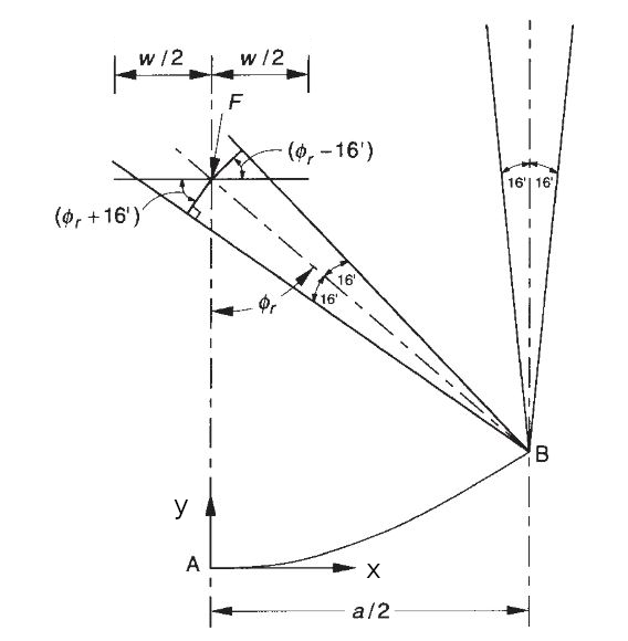 Rim Angle diagram from Duffie and Beckman. 16’= $0.267 ^{\circ}$ is the half-angle subtended by the Sun $\theta_s$, $a$ is the diameter of the aperature (mirror), and $D$ (not shown) is the diameter of the receiver (rocket)
For a perfect parabolic or parabaloidal mirror, the Diameter D of the receiver is given by the equation: \(D={a sin(\theta_s) \over sin(\phi_r)}\)
We can then rewrite the concentration ratio as:
\[C={(\pi/4) a^2 \over (\pi/4) D^2} = {a^2 \over D^2}\]To find the focal length and aperature diameter with the maximum concentration ratio, we can either simplify the above equation in terms of $a$ and $f$ and calculate the gradient or plot the concentration ratio as a function of focal length and aperature diameter (the latter is more illustrative):
1
2
3
4
5
6
7
8
9
10
11
12
13
14
15
16
17
18
19
20
21
import numpy as np
import matplotlib.pyplot as plt

theta_s = 0.267 * (np.pi/180)

fig,ax=plt.subplots(2,2) #Create 4 plots and show that the maximum concentration ratio occurs at aperature = 4x focus
f_s=np.asarray((10**3, 10**4, 10**5, 3*10**5))
for i in range(2):
    for j in range(2):
        f = f_s[i+j]
        a = np.linspace(0.1,f*5,10**4)
        phi_r = np.arctan((a/2)/(f-(1/(4*f))*(a/2)**2))
        D = a*np.sin(theta_s)/np.sin(phi_r)
        C=a**2/D**2
        ax[i,j].plot(a,C,label='$F = 10^'+str(int(np.log10(f)))+'$ [m]')
        ax[i,j].legend()
        ax[i,j].set_xlabel('Aperature Diameter [m]')
        ax[i,j].set_ylabel('Concentration Ratio')
        ax[i,j].ticklabel_format(style='sci')
fig.tight_layout()
plt.show()
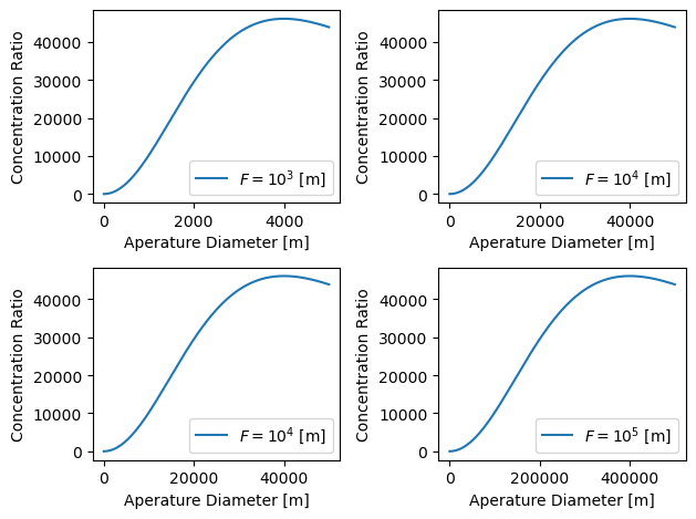 Concentration Ratio as a function of Aperature Diameter for a fixed Focal Length
1
2
3
4
5
6
7
8
9
10
11
12
13
14
15
16
17
18
19
20
21
22
23
24
25
26
import numpy as np
import matplotlib.pyplot as plt

theta_s = 0.267 * (np.pi/180)

f = np.linspace(0.1,3*10**5,10**3)
a = np.linspace(0.1,3*10**5,10**3)
F, A = np.meshgrid(f,a)
phi_r = np.arctan((A/2)/(F-(1/(4*F))*(A/2)**2))
D = A*np.sin(theta_s)/np.sin(phi_r)
C=A**2/D**2

fig,ax=plt.subplots(1,1)
cp = ax.contourf(F,A,C)
fig.colorbar(cp) # Add a colorbar to a plot
ax.plot(f,4*f,label='a=4f',color='red',linestyle='dashed')
ax.plot(f,2*f,label='a=2f',color='maroon',linestyle='dashed')
ax.plot(f,f,label='a=f',color='orange',linestyle='dashed')
ax.plot(f,f/2,label='a=f/2',color='yellow',linestyle='dashed')
ax.set_ylim(0,f[-1])
ax.legend()
ax.set_title('Concentration Ratio')
#ax.set_xlabel('x (cm)')
ax.set_ylabel('Aperature Diameter [m]')
ax.set_xlabel('Focal Length [m]')
plt.show()
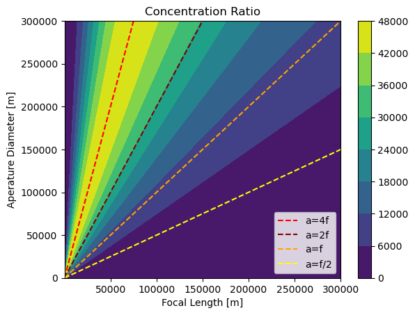 Concentration Ratio as a function of Aperature Diameter and Focal Length
From these graphs, we can see that if you want the highest concentration ratio possible, the aperature diameter $a$ must be 4 times larger than the focal distance. This means that for one large parabolic mirror, the height of the rim of your mirror must be $y={1 \over 4f}x^2={1 \over 4f}(a/2)^2={1 \over 4f}(4f/2)^2=f$. More practically, following the concept of a fresnel lens or solar power tower, it would be better to have a series of concentric arrays of multiple smaller mirrors, varying the focal distance and normal angle as a function of their radial position $x$ from the center of the mirror array according to the following equations:
\[f(x) = \sqrt{f_{0}^2+x^2}\] \[\theta_{n}(x)={tan^{-1}({x \over f_{0}}) \over 2}\]where $f_{0}$ is the focal distance at the center of the mirror array. Regardless, this would still mean that the diameter of the mirror array would need to be at least 2-4 times larger than the focal distance (~150-300 [km]) for the concentration ratios required.
A series of balloon-based or space-based mirror arrays made of mylar could reduce the distance between the mirrors and the rocket but at the expense of significantly more system complexity. Additionally, this analysis didn’t account for the cosine losses as the rocket moves accross each mirror array field, atmospheric attenuation (which could be assumed to be on the order of ~300 [W/$m^2$] given the difference between the extraterrestrial solar constant and the DNI measured on the ground), mirror reflectivity and soiling losses, deviations from a perfect parabolic shape, and tracking errors.
Solar “Lasers” are Impossible
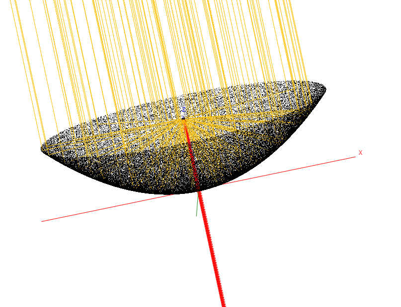
One last aside: a few years ago, I briefly thought it would be possible to create a solar “laser” by placing a smaller parabola at the focus of the larger parabola (see subsequent figures). Assuming the light from the sun is perfectly collimated (parallel), this might be an effective way to control a beam of concentrated sunlight - also assuming the mirror didn’t melt. However, as you can see from the plotted rays in SolTrace, if you account for the actual shape of the sun and the real direction of the suns rays, the concentrated solar “beam” has an angular spread proportional to the ratio of the cross-sectional areas of the parabolic mirrors.
 A Solar “Laser” assuming sunlight is perfectly collimated/parallel
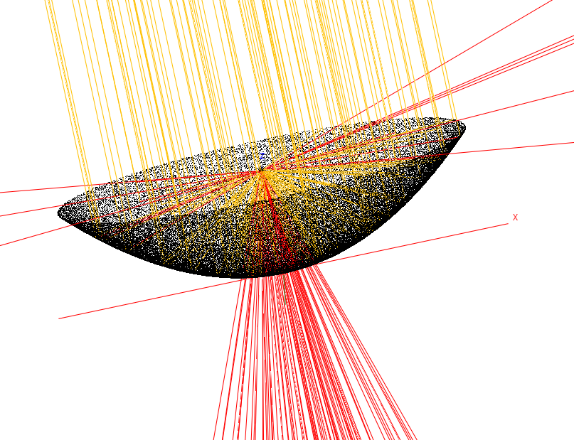 The Solar “Laser” not working because of the real shape of the sun
Minimum Required Concentration Ratio Neglecting Focal Distance
Assuming the temperature requirements are 1500 [K] and 300 [MW] of power delivered, the following equation can be used to find the required concentration ratio for a given vehicle cross-sectional area (assuming it’s close to blackbody):
\[q_{in}-q_{out}=300*10^6 [W]=A\dot{q}_{sol}C-\sigma A(T_{rocket}^4-T_{\inf}^4)\]Varying the cross-sectional area $A$, we can plot the minimum concentration ratio:
1
2
3
4
5
6
7
8
9
10
11
12
13
14
15
16
17
import matplotlib.pyplot as plt
import numpy as np

T_inf = 300 #[K]
T_rocket = 1500 #[K]
sigma = 5.67*10**-8
q_sol = 1337 #[W/m^2]
A = np.linspace(0.1,1000,1000) #[m]
w=A**(1/2)
q_rocket = 300*10**6 #[m]
C=(q_rocket+sigma*A*(T_rocket**4-T_inf**4))/(q_sol*A)
plt.semilogy(A,C)
plt.ylabel("Concentration Ratio")
plt.xlabel("Receiver Area [$m^2$]")
plt.ylim(0,48000)
plt.title("$T_{rocket}$=%i[K], $\dot{q}_{rocket}=%i$ [W]"%(T_rocket,q_rocket))
plt.show()
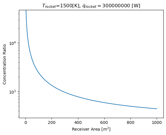 Concentration Ratio as a function of A for T=1500[K] and q=300[MW]
Neglecting focal distance, we can see that for a very large heat exchanger area of 200 [$m^2$], this yields a concentration ratio of ~1300 and a field area of 270,000 [$m^2$], which is fairly close to numbers for a commercial solar power tower. If somehow instead of beaming the energy, the rocket carried its own optics, this might be more feasible (although still pretty infeasible).
Conclusion
While it is theoretically possible to heat a rocket at a distance using solar energy, it is fairly impractical given the precision and shear size of the mirror arrays required even under perfect conditions. One might have better luck launching something above the atmosphere, where air resistance is extremely low, and using an onboard highly precise fresnel lens or lenses or a trailing parabolic mirror or array of mirrors to accelerate a very small vehicle to orbital speeds. Additionally, the breakthroughs in the field of non-imaging optics were not discussed in this article but further reading can be done in The Optics of Nonimaging Concentrators by Welford and Winston. This analysis also did not account for the spillage of the beam and the potential to damage surrounding satellites and aircraft.
How to Cite
BibTeX
@www{mullinsolar2023, title = {Analysis of a Solar Thermal Beam-Powered Propulsion Rocket}, author = {Mullin, M}, year = {2023}, url = {https://www.matthewjmullin.com/posts/solar-rocket/}, urldate = {2.20.23}, }
APA:
Mullin, M. Analysis of a Solar Thermal Beam-Powered Propulsion Rocket. https://www.matthewjmullin.com/posts/solar- rocket/, accessed on 2.20.23.